Online Mode: Implementation Guide

We recommend to check first the PDAF Tutorials, which provide an easy step-by-step description for assimilation program in the offline and oneline modes utilizing example tutorial codes. The Implementation Guide provides more details, e.g. descriptions of the defined interfaces, but is less applied.

This page contains the implementation guide for the online mode of PDAF in which PDAF is attached to the numerical model. For the offline mode, in which separate programs for model integrations and assimilation step are executed, see the Implementation Guide for the Offline Mode. The differences between the online and offline modes is described on the page on the Implementation concept of PDAF.

Note: This Implementation Guide explains the implementation as of PDAF V3. The recommendations differ from those for PDAF 2. For reference, for implementations that were done for PDAF 2, the Implementation Guide for PDAF 2 is still available.

The implementation of PDAF with an existing model

For the online data assimilation mode of PDAF, the numerical model has to be combined with PDAF into a single program to generate the assimilation system. This is done by adding several subroutine calls into the model code.

Examples of the implementation are given in tutorial code provided with PDAF in tutorial/online_2D_serialmodel and tutorial/online_2D_parallelmodel. These examples base on the template code at templates/online. Several subroutines that contain specific operations for the model and observations are called by PDAF through its defined interface as call-back routines. These subroutines need to be implemented by the user. The operations in all these subroutines are rather elementary like filling the array of the ensemble of model states from model output files and the initialization of the vector of observations. The tutorial code includes examples for these routines for a simple case.

We recommend to base your own implementation on the template by utilizing the provided PDAF-specific routines and inserting them to your model.

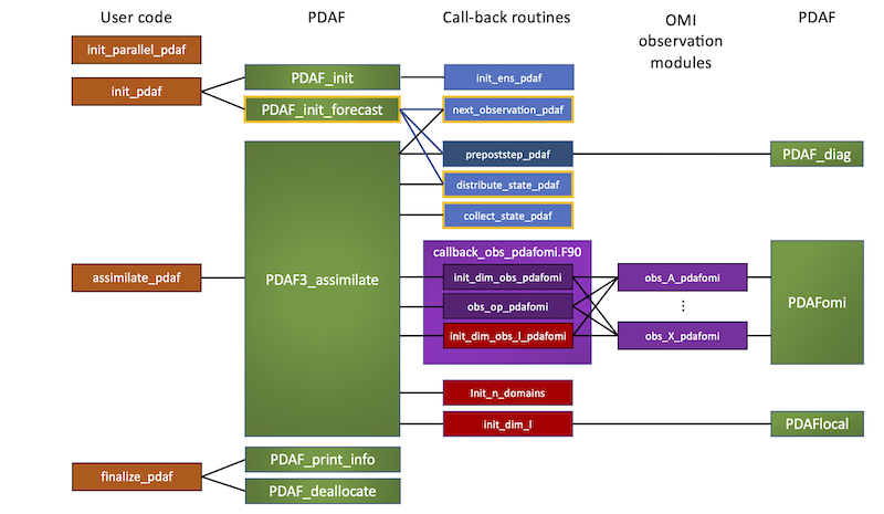
Figure 1 provides an overview of the call structure of the offline code.

Figure 1: Overall call structure in PDAF's online mode. Boxes with orange frame show subroutines that are specific for the online mode and not not in the offline mode.

The code structure is as follows from left to right

• column 1 'User code': The model code calls the four routines shown in this column. These are interface routines, which define variables for PDAF and then call core-subroutines of PDAF. An exception is init_parallel_pdaf which does not call PDAF. The calls to these routines are added to the model source code.
• column 2 'PDAF': These are the PDAF core routines which are called by the routines in column 1 to the left.
• column 3 'Call-back routines': This column shows the call-back routines, which are called by the PDAF routines in column 2 to the left. The routines in the purple box callback_obs_pdafomi.F90 are the subroutines that handle observations. The 3 routines in red are used only for localized ensemble filters.
• column 4 'OMI observation modules': This column shows observation modules that are used for the specific handling of each observation type. This handling is arranged by the PDAF Observation Module Interface (OMI). The observation-related call-back routines in column 3 to the left call routines in each of the observation modules.
• column 5 'PDAF': Some of the call-back routines and the routines in the observation modules call PDAF core routines, e.g. for diagnostics, localization, and to intialize OMI.

The implementation of the assimilation program for PDAF in offline mode can be performed in following the four routines in the leftmost column:

1. init_parallel_pdaf: Adapting the parallelization
2. init_pdaf: Initializing PDAF
3. assimilate_pdaf (Part 1): Modifying the model code for the ensemble integration
4. assimilate_pdaf (Part 2): Implementing the analysis step
5. finalize_pdaf: Adding memory and timing information

The names of PDAF core routines always start with PDAF. The subroutines with name ending _pdaf are generally user-supplied routines in the tutorial codes. An overview of the available options for each filter that can be specified when PDAF is initialized is given on the overview page on options.

Generating initial ensembles

To perform ensemble data assimilation one has to create an initial ensemble which is then used in the data assimilation process. There are various different ways to generate an ensemble (like random picking of model states, breeding, short-term integrations of perturbed model fields, second-order exact sampling from EOFs). PDAF provides routines to use snapshots from a model integration to first compute EOFs (empirical orthogonal functions) and then to use the EOFs to perform a constrained random transformation to obtain ensemble perturbations to which a central state (i.e. ensemble mean) is added. This second-order exact sampling (Pham, 2001) showed good performance in our own data assimilation applications.

The ensemble generation is described on the separate page:

1. Ensemble Generation