Implementation Concept of the Online Mode

Online mode: Attaching PDAF to a model

Here we describe the extensions of the model code for the online mode of PDAF.

The assimilation system is built by adding call to PDAF-routines to the general part of the model code. As only minimal changes to the model code are required, we refer to this as "attaching" PDAF to the model.

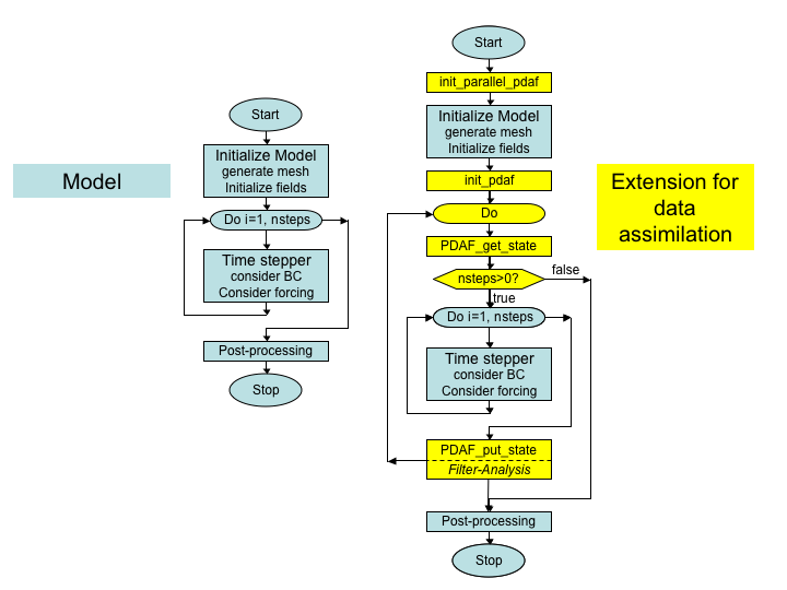
The general concept is depicted in figure 1. The left hand side shows a typical abstract structure of a numerical model. When the program is executed, the following steps are performed:

1. The model is initialized. Thus arrays for the model fields are allocated and filled with initial fields. Thus, the model grid is build up virtually in the program.
2. After the initialization the time stepping loop is performed. Here the model fields are propagated through time.
3. When the integration of the model fields is completed after a defined number of time steps, various post-processing operations are performed. Then the program stops.

Figure 1: (left) Generic structure of a model code, (right) extension for data assimilation with PDAF

The right hand side of Figure 1 shows the extensions required for the assimilation system (marked yellow):

• init_parallel_pdaf: This routine is inserted close to the start of the model code. If the model itself is parallelized the correct location is directly after the initialization of the parallelization in the model code. init_parallel_pdaf creates the parallel environment that allows to perform several time stepping loops ("model tasks") at the same time.
• init_pdaf: This routine is added after the initialization part of the model. In init_pdaf, parameters for PDAF can be defined and then the core initialization routine PDAF_init is called. This core routine also initializes the array of ensemble states.
• Ensemble loop: In order to allow for the integration of the state ensemble an unconditional loop is added around the time stepping loop of the model. This loop will allow to compute the time stepping loop multiple time during the model integration. PDAF provides an exit-flag for this loop. (There are some conditions, under which this external loop is not required. Some notes on this are given further below.)
• PDAF_get_state: Inside the ensemble loop, the PDAF core routine PDAF_get_state is added to the code. This routine initializes model fields from the array of ensemble states and initializes the number of time steps that have to be computed and ensures that the ensemble integration is performed correctly.
• PDAF_put_state: At the end of the external loop, the PDAF core routine PDAF_put_state is added to the model code. This routine writes the propagated model fields back into a state vector of the ensemble array. Also it checks whether the ensemble integration is complete. If not, the next ensemble member will be integrated. If the ensemble integration is complete, the analysis step (i.e. the actual assimilation of the observations) is computed.

With the implementation strategy of PDAF, four routines and the external loop have to be added to the model code. While this looks like a large change in figure 1, this change does actually only affect the general part of the model code. In addition, the amount of source code of the numerical model will be much longer than the addition for the data assimilation system.

Important aspects of the implementation concept

• The implementation concept of PDAF does not require that the time stepping part of the model is implemented as a subroutine. Instead calls to subroutines that control of the ensemble integration are added to the model code before and after the code parts performing the time stepping. If the time stepping part is implemented as a subroutine, this subroutine can be called in between the additional routines.
• Depending on the parallelization, there can be cases in which the model has to jump back in time and cases in which the time always moves forward:
  • Jumping back in time will be required if the number of model tasks used to evolve the ensemble states is smaller than the number of ensemble members. In this case a model task has integrate more than one model state and will have to jump back in time after the integration of each ensemble member.
  • If there are as many model tasks as ensemble members, the model time always moves forward. In this case, one can implement PDAF also without the external ensemble loop. That is, one can add calls to PDAF_get_state and PDAF_put_state directly into the code of the model's time stepping loop. This strategy might also be called for, if a model uses nested loops (like a loop over minutes inside a loop over hours).
• Model-specific operations like the initialization of the array of ensemble states in PDAF_init are actually performed by user-supplied routines. These routines are called through the standard interface of PDAF. Details on the interface and the required routines are given on the pages describing the implementation steps.
• The assimilation system is controlled by the user-supplied routines that are called through PDAF. With this strategy, the assimilation program is essentially driven by the model part of the program. Thus, logically the model is not a sub-component of the assimilation system, but the implementation with PDAF results in a model extended for data assimilation.
• The user-supplied routines can be implemented analogously to the model code. For example, if the model is implemented using Fortran common blocks or modules of the model code, these can be used to implement the user-supplied routines, too. This simplifies the implementation of the user-supplied routines knowing about the particularities of their model.

Parallelization of the data assimilation program

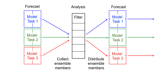
PDAF adds the possibility to perform parallel ensemble forecasts, even for models that by themselves do not use parallelization. The structure of the parallelized data assimilation program is displayed in figure 2. In the forecast phase of the data assimilation application, several model state integrations can be performed at the same time by several model tasks. If the numerical model it parallelized by itself, the parallel ensemble forecast adds a second level of parallelization. For the analysis step, in which the filter combines the ensemble of model states with the observations, PDAF provides several parallelized filter algorithms. If the model uses domain decomposition for the parallelization, the same decomposition is typically used in the filter. Before the analysis step, all ensemble members are gathered by the processes that compute the filter analysis. Subsequently to the analysis step, the ensemble members are distributed to all model tasks to enable the next parallel ensemble forecast. These operations are performed within PDAF, so that a user can directly benefit from the second level of parallelization. For the required extension of the parallelization configuration of the model a fully implemented template routine is provided with PDAF. The adaptation of the parallelization is described in the Implementation Guide.

Figure 2: Two-level parallelization of PDAF: During the forecast phase several model tasks can be concurrently performed, while each model can be parallelized by itself. In the analysis step one the parallelized filter included in PDAF is applied.