Implementation Concept of the Online Mode

Online mode: Attaching PDAF to a model

Here we describe the extensions of the model code for the online mode of PDAF. We focus here on the fully-parallel implementation variant. For this variant, we assume that there is a sufficient number of processes when running the data assimilation program so that all ensemble states can be propagated concurrently. In this case, the model always runs forward in time and the implementation of the data assimilation with PDAF only requires the addition of some subroutine calls.

The second implementation variant, called flexible parallel, allows to run the assimilation program in a way so that a model task (set of processors running one model integration) can propagate several ensemble states successively. This implementation variant is a bit more complicated, because one has to ensure that the model can jump back in time. We discuss the ''flexible parallel'' variant further below.

If the data assimilation can be run with a sufficient number of processors to use the fully-parallel variant, we recommend to use it. With today's compute clusters with a large number of processors, this approach is usually possible.

Fully-parallel implementation

The assimilation system is built by adding subroutine calls to the general part of the model code. In these routines one can define variables for PDAF, use-include the PDAF module and call the PDAF core subroutines. Usually only single lines with a subroutine call are inserted into the model code. Because only minimal changes to the model code are required, we refer to this as "attaching" PDAF to the model.

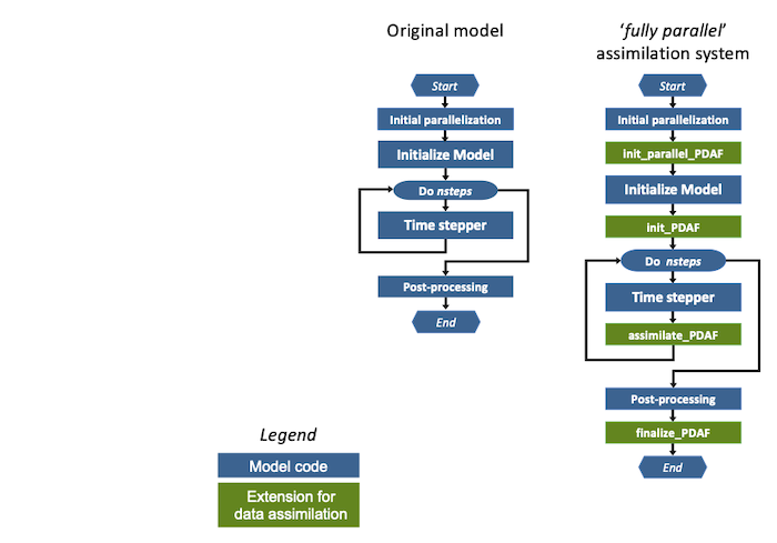
The general concept is depicted in figure 1. The left hand side shows a typical abstract structure of a model. When the program is executed, the typical steps done in the program are the following:

1. The model might intialize parallelization
2. The model is initialized. Thus, model fields arrays are allocated and filled with initial fields. Thus, the model grid is build up virtually in the program.
3. The time stepping loop is performed over isteps time steps. Here the model fields are propagated through time.
4. After time stepping, post-processing operations can be performed. This usually includes file output, e.g. writing restart files. Afterwards, the program stops.

Figure 1: (left) Generic structure of a model code, (right) modified structure for fully-parallel data assimilation system with PDAF. The figure assumes that the model is parallelized, such that it initializes its parallelization in the step Initial parallelization. If the model is not parallelized this step does not exist.

Extensions for the fully-parallel assimilation system
The right side of Figure 1 shows the extensions required for the fully-parallel assimilation system (marked green):

• init_parallel_pdaf: This subroutine is inserted close to the start of the model code. If the model itself is parallelized the correct location is directly after the initialization of the parallelization in the model code. init_parallel_pdaf creates the parallel environment that allows to compute the time stepping for an ensemble of models ("model tasks") at the same time.
• init_pdaf: This subroutine is added after the initialization part of the model, just before the time stepping loop. In this subroutine one defines parameters for PDAF and then one calls the core initialization routine PDAF_init. This core routine initializes internal parameters and afterwards the array of ensemble states using a user-provided call-back routine. Subsequently, one calls the PDAF core routine PDAF_init_forecast (in implementations of PDAF before version 3.0, this routine was called PDAF_get_state). This routine initializes model fields from the array of ensemble states using a call-back routine. In addition, it returns the number of time steps that have to be computed in the following forecast phase.
• assimilate_pdaf: This routine is added to the model code into the time stepper before the end of the time stepping loop (usually just before the END DO in a Fortran program). The routine declares the names of user-supplied subroutines and calls a PDAF-core routine like PDAF3_assimilate. (In implementations of PDAF before version 3.0, different routines named PDAFomi_assimilate_X with, e.g., X=local, for local filters are used). This routine has to be called at the end of each time step. It counts whether all time steps of the current forecast phase have been computed. If this is not the case, the program continues integrating the model. If the forecast phase is completed, the analysis step, i.e. the actual assimilation of the observations, is computed. Subsequently, the next forecast phase is initialized by writing the analysis state vector into the model fields and setting the number of time steps in the next forecast phase.
• finalize_pdaf: This routine is used to let PDAF display timing and memory information and to call PDAF to deallocate its internal arrays.

With the implementation strategy of PDAF, calls to four subroutines are added to the model code. These additions are usually only single lines of code and the changes only affect the general part of the model code.

A code example for the fully parallel mode is provided in the tutorial code in tutorial/online_2D_serialmodel. See also the PDAF implementation tutorial.

Important aspects of the implementation concept

• The implementation concept of PDAF attaches the data assimilation functionality to the model. With this approach, the model with attached data assimilation is finally run analogous to a normal model run, but with additional processors and additional options for the data assimilation.
• The implementation with PDAF does not require that the time stepping part of the model is implemented as a subroutine. Instead calls to subroutines that control the the ensemble integration are added to the model code. This minimizes the changes in the model code.
• In the fully parallel mode described here, we use as many model tasks as ensemble members. Thus, the model always moves forward in time.
• PDAF uses the concept to 'pull' information at the time when it is needed. All model-specific operations, like the initialization of the array of ensemble states in PDAF_init, are performed by user-supplied routines which are called through PDAF's standard interface as call-back routines. Also the reading of observational infromation is performed by user-supplied call-back subroutines. Details on the interface and the required routines are given on the pages describing the implementation steps. The concept of the call-back routines is depicted in Fig. 2.
• The assimilation system is controlled by the user-supplied routines that are called through PDAF as call-back routines. With this strategy, the assimilative model program is essentially driven by the model part of the program. Thus, the model is not a sub-component of the assimilation system, but the implementation with PDAF results in a model extended for data assimilation.
• The user-supplied call-back routines can be implemented in the context of the model analogously to the model code. For example, if the model is implemented using Fortran modules (or even common blocks), these can be used to implement the user-supplied routines, too. This simplifies the implementation of the user-supplied routines knowing about the particularities of their model.

Figure 2: Use of user-supplied call-back functions in PDAF. The call-back routines are called by PDAF and can use model information that is provided by Fortran modules.

Parallelization of the data assimilation program

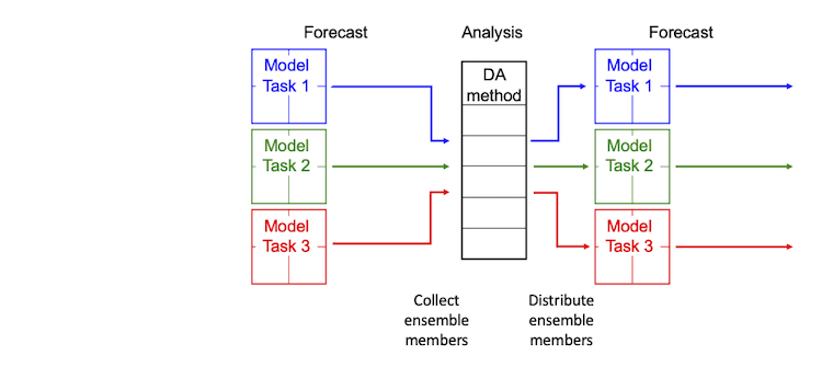
PDAF adds the possibility to perform parallel ensemble forecasts, even for models that by themselves do not use parallelization. The structure of the parallelized data assimilation process is displayed in Figure 3. In the forecast phase of the data assimilation application, several model tasks can perform model state integrations at the same time. If the numerical model it parallelized by itself, the parallel ensemble forecast adds a second level of parallelization. For the analysis step, in which the DA method combines the ensemble of model states with the observations, PDAF provides several parallelized DA methods. If the model uses domain decomposition for the parallelization, the same decomposition is typically used in the DA method. Before the analysis step, all ensemble members are gathered by the processes that compute the filter analysis. Subsequently to the analysis step, the ensemble members are distributed to all model tasks to enable the next parallel ensemble forecast. These operations are performed within PDAF, so that a user can directly benefit from the second level of parallelization. For the required extension of the parallelization configuration, a fully implemented template routine is provided with PDAF. The adaptation of the parallelization is described in the [ImplementationGuide_PDAF3 Implementation Guide].

Figure 3: Two-level parallelization of PDAF: During the forecast phase several model tasks compute model integrations concurrently, while each model can be parallelized by itself, e.g., using domain decomposition (colored boxes). For the analysis step one the parallelized data assimilation methods included in PDAF is applied.

Flexible parallel implementation

Note: This description is for the updated structure that introduced with PDAF V3.0. Implementations for PDAF V2 followed the former structure which is described on the Page on the flexible parallelization mode in PDAF2.

The flexible parallel mode allows to run the assimilation program in a way so that a model task can propagate several ensemble states on after the other. This approach allows one to use a smaller number of processes compared to the fully parallel. In the extreme case, a single model task can integrate all ensemble states.

The flexible parallelization requires that the model can jump back in time. If the number of model tasks used to evolve the ensemble states is smaller than the number of ensemble members, each model task propagates more than one model state. In this case, a model task has integrate more than one model state. Thus, it will have to jump back in time after the integration of each ensemble member, in order to integrate the next state over the same time period.

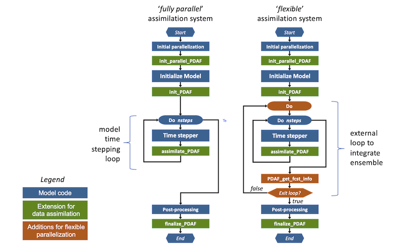
Implementing the flexible mode requires additional changes to the model code. These are shown in Figure 4. In particular an external loop has to be added. In addition, a call to PDAF_get_fcst_info determines the number of time steps for the net forecast phase.

Figure 4: Extension for flexible parallel data assimilation system. The right hand side shows the structure for the fully parallel mode, while the orange parts are the modifications for the flexible parallel mode.

Extensions for the flexible assimilation system
Figure 4 shows the extensions required for the flexible assimilation system (marked green with additional changes compared to the fully parallel mode marked orange):

• init_parallel_pdaf: This routine is inserted close to the start of the model code in the same way as for the fully parallel mode.
• init_pdaf: This routine is added after the initialization part of the model in the same way as for the fully parallel mode. The routine also determines the number of time steps for the initial forecast phase.
• Ensemble loop: In order to allow for the integration of the state ensemble, an unconditional loop is added around the time stepping loop of the model. This loop will allow to compute the time stepping loop multiple times to integrate all ensemble states. PDAF_get_fcst_info provides an exit flag for this loop, which is checked to control when to exit this loop.
• PDAF_get_fcst_info: The call to PDAF_get_fcst_info is used to obtain the number of time steps (nsteps) for the next forecast phase and the value of the exit flag. Subsequently, one checks the exit flag and when this indicates to end the assimilation process, one steps out of the outer unconditional loop. Otherwise, the program continues with the next forecast phase.
• assimilate_pdaf: Inside the ensemble loop, a call to this interface routine is added to the code in the same way as for the fully parallel mode.
• finalize_pdaf: This routine is added to the code in the same way as for the fully parallel mode.

A code example for the flexible mode is provided in the template codes in templates/online_flexible/.