The flexible parallelization mode in PDAF2

With PDAF V3.0 we changed the recommended code structure for the flexible parallelization mode. Here, we show the structe that was used in PDAF V2.3.1 and before.

The flexible parallelization mode allows to run the assimilation program in a way so that a model task (set of processors running one model integration) can propagate several ensemble states successively. This approach allows to use a smaller number of processes compared to the fully parallel'.

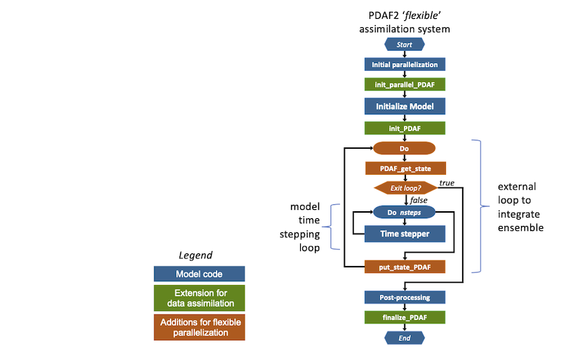
Implementing the flexible mode requires additional changes to the model code. These are shown in Figure 1. In particular an external loop has to be added. This change only affects the general part of the model code. Compared to the newer implementation variant, a combination of calls to PDAF_get_state and put_state_PDAF (which calls PDAFomi_put_state_X or PDAF_put_state_X for a specific DA-method 'X') is used. In this case, put_state_PDAF is called after the full integration of an ensemble member state. Then PDAFomi_put_state_X counts the number of ensemble members for which the forecast is complete. If all members were integrated, the analysis step is executed to compute the assimilation update. This structure does not allow to perform additional operations during the time stepping like apply incremental analysis updates. In contrast the recommended implementation introduced with PDAF V3.0, performs a call to PDAF at each time step.

The flexible parallelization requires that the model can jump back in time. Jumping back in time will be required if the number of model tasks used to evolve the ensemble states is smaller than the number of ensemble members. In this case a model task has integrate more than one model state and will have to jump back in time after the integration of each ensemble member.

Figure 1: Extension for flexible data assimilation system with PDAF V2.3.1 and before.

Extensions for the flexible assimilation system for PDAF V2.3.1 and before
Figure 1 shows the extensions required for the flexible assimilation system (marked yellow):

• init_parallel_pdaf: This routine is inserted close to the start of the model code. If the model itself is parallelized the correct location is directly after the initialization of the parallelization in the model code. init_parallel_pdaf creates the parallel environment that allows to perform several time stepping loops ("model tasks") at the same time.
• init_pdaf: This routine is added after the initialization part of the model. In init_pdaf, parameters for PDAF can be defined and then the core initialization routine PDAF_init is called. This core routine also initializes the array of ensemble states.
• Ensemble loop: In order to allow for the integration of the state ensemble, an unconditional loop is added around the time stepping loop of the model. This loop will allow to compute the time stepping loop multiple times to integrate all ensemble states. PDAF provides an exit-flag for this loop. (This external loop is avoided with the fully-parallel implementation variant.)
• get_state_pdaf: Inside the ensemble loop, a call to this interface routine is added to the code. In this routine the names of user-supplied routines are declared and the PDAF-core routine PDAF_get_state is called. This routine initializes model fields from the array of ensemble states and initializes the number of time steps that have to be computed and ensures that the ensemble integration is performed correctly.
• put_state_pdaf: At the end of the external loop, the call to the interface routine put_state_pdaf is added to the model code. The routine declares the names of user-supplied routines and calls a PDAF_core routine that is specific for the DA methods. E.g., the routine PDAFomi_put_state_local is called for the local ensemble Kalman filters. This routine writes the propagated model fields back into a state vector of the ensemble array. Also it checks whether the ensemble integration is complete. If not, the next ensemble member will be integrated. If the ensemble integration is complete, the analysis step (i.e. the actual assimilation of the observations) is computed.